Macro codes can save you a ton of time. You can automate small as well as heavy tasks with VBA codes.
And do you know? With the help of macros, you can break all the limitations of Excel which you think Excel has.
And today, I have listed some of the useful codes examples to help you become more productive in your day to day work.
You can use these codes even if you haven’t used VBA before that. But here’s the first thing to know:
In Excel, macro code is a programming code which is written in VBA (Visual Basic for Applications) language. The idea behind using a macro code is to automate an action which you perform manually in Excel, otherwise.
For example, you can use a code to print only a particular range of cells just with a single click instead of selecting the range > File Tab > Print > Print Select > OK Button.
Before you use these codes, make sure you have your developer tab on your Excel ribbon to access VB editor. Once you activate developer tab you can use below steps to paste a VBA code into VB editor.
Learn VBA in 1 Hour
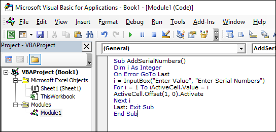
This macro code will automatically add serial numbers to your Excel sheet, which can be helpful if you work with large amounts of data.
Sub AddSerialNumbers()
Dim i As Integer
On Error GoTo Last
i = InputBox("Enter Value", "Enter Serial Numbers")
For i = 1 To i
ActiveCell.Value = i
ActiveCell.Offset(1, 0).Activate
Next i
Last:Exit Sub
End Sub
To use this code, you need to select the cell from where you want to start the serial numbers and when you run this it shows you a message box where you need to enter the highest number for the serial numbers and click OK.
And once you click OK, it simply runs a loop and add a list of serial numbers to the cells downward.
This code helps you to enter multiple columns in a single click.
Sub InsertMultipleColumns()
Dim i As Integer
Dim j As Integer
ActiveCell.EntireColumn.Select
On Error GoTo Last
i = InputBox("Enter number of columns to insert", "Insert Columns")
For j = 1 To i
Selection.Insert Shift:=xlToRight, CopyOrigin:=xlFormatFromRightorAbove
Next j
Last: Exit Sub
End Sub
When you run this code, it asks you the number columns you want to add and when you click OK, it adds entered number of columns after the selected cell. If you want to add columns before the selected cell, replace the xlToRight to xlToLeft in the code.
With this code, you can enter multiple rows in the worksheet. When you run this code, you can enter the number of rows to insert and make sure to select the cell from where you want to insert the new rows.
Sub InsertMultipleRows()
Dim i As Integer
Dim j As Integer
ActiveCell.EntireRow.Select
On Error GoTo Last
i = InputBox("Enter number of columns to insert", "Insert Columns")
For j = 1 To i
Selection.Insert Shift:=xlToDown, CopyOrigin:=xlFormatFromRightorAbove
Next j
Last: Exit Sub
End Sub
If you want to add rows before the selected cell, replace the xlToDown to xlToUp in the code.
This code quickly auto fits all the columns in your worksheet.
Sub AutoFitColumns()
Cells.Select
Cells.EntireColumn.AutoFit
End Sub
When you run this code, it will select all the cells in your worksheet and instantly auto-fit all the columns.
You can use this code to auto fit all the rows in a worksheet.
Sub AutoFitRows()
Cells.Select
Cells.EntireRow.AutoFit
End Sub
When you run this code, it will select all the cells in your worksheet and instantly auto fit all the rows.
This code will help you to remove text wrap from the entire worksheet with a single click.
Sub RemoveTextWrap()
Range("A1").WrapText = False
End Sub
It will first select all the columns and then remove text wrap and auto fit all the rows and columns. There’s also a shortcut that you can use (Alt + H +W) for but if you add this code to Quick Access Toolbar it’s convenient than a keyboard shortcut.
This code simply uses the unmerge options which you have on the HOME tab.
Sub UnmergeCells()
Selection.UnMerge
End Sub
The benefit of using this code is you can add it to the QAT and unmerge all the cell in the selection. And if you want to un-merge a specific range you can define that range in the code by replacing the word selection.
In Windows, there is a specific calculator and by using this macro code you can open that calculator directly from Excel.
Sub OpenCalculator()
Application.ActivateMicrosoftApp Index:=0
End Sub
As I mentioned that it’s for windows and if you run this code in the MAC version of VBA you’ll get an error.
This macro adds a date to the header when you run it. It simply uses the tag “&D” for adding the date.
Sub DateInHeader()
With ActiveSheet.PageSetup
.LeftHeader = ""
.CenterHeader = "&D"
.RightHeader = ""
.LeftFooter = ""
.CenterFooter = ""
.RightFooter = ""
End With
End Sub
You can also change it to the footer or change the side by replacing the “” with the date tag. And if you want to add a specific date instead of the current date you can replace the “&D” tag with that date from the code.
When you run this code, it shows an input box that asks you to enter the text which you want to add as a header, and once you enter it click OK.
Sub CustomHeader()
Dim myText As String
myText = InputBox("Enter your text here", "Enter Text")
With ActiveSheet.PageSetup
.LeftHeader = ""
.CenterHeader = myText
.RightHeader = ""
.LeftFooter = ""
.CenterFooter = ""
.RightFooter = ""
End With
End Sub
If you see this closely you have six different lines of code to choose the place for the header or footer. Let’s say if you want to add left-footer instead of center header simply replace the “myText” to that line of the code by replacing the “” from there.
These VBA codes will help you to format cells and ranges using some specific criteria and conditions.
This macro will check each cell of your selection and highlight the duplicate values. You can also change the color from the code.
Sub HighlightDuplicateValues()
Dim myRange As Range
Dim myCell As Range
Set myRange = Selection
For Each myCell In myRange
If WorksheetFunction.CountIf(myRange, myCell.Value) > 1 Then
myCell.Interior.ColorIndex = 36
End If
Next myCell
End Sub
I really love to use this macro code whenever I have to analyze a data table.
Private Sub Worksheet_BeforeDoubleClick(ByVal Target As Range, Cancel As Boolean)
Dim strRange As String
strRange = Target.Cells.Address & "," & _
Target.Cells.EntireColumn.Address & "," & _
Target.Cells.EntireRow.Address
Range(strRange).Select
End Sub
Here are the quick steps to apply this code.
Remember that, by applying this macro you will not able to edit the cell by double click.
Just select a range and run this macro and it will highlight top 10 values with the green color.
Sub TopTen()
Selection.FormatConditions.AddTop10
Selection.FormatConditions(Selection.FormatConditions.Count).S
tFirstPriority
With Selection.FormatConditions(1)
.TopBottom = xlTop10Top
.Rank = 10
.Percent = False
End With
With Selection.FormatConditions(1).Font
.Color = -16752384
.TintAndShade = 0
End With
With Selection.FormatConditions(1).Interior
.PatternColorIndex = xlAutomatic
.Color = 13561798
.TintAndShade = 0
End With
Selection.FormatConditions(1).StopIfTrue = False
End Sub
If you are not sure about how many named ranges you have in your worksheet then you can use this code to highlight all of them.
Sub HighlightRanges()
Dim RangeName As Name
Dim HighlightRange As Range
On Error Resume Next
For Each RangeName In ActiveWorkbook.Names
Set HighlightRange = RangeName.RefersToRange
HighlightRange.Interior.ColorIndex = 36
Next RangeName
End Sub
Once you run this code it will ask you for the value from which you want to highlight all greater values.
Sub HighlightGreaterThanValues()
Dim i As Integer
i = InputBox("Enter Greater Than Value", "Enter Value")
Selection.FormatConditions.Delete
Selection.FormatConditions.Add Type:=xlCellValue, _
Operator:=xlGreater, Formula1:=i
Selection.FormatConditions(Selection.FormatConditions.Count).S
tFirstPriority
With Selection.FormatConditions(1)
.Font.Color = RGB(0, 0, 0)
.Interior.Color = RGB(31, 218, 154)
End With
End Sub
Once you run this code it will ask you for the value from which you want to highlight all lower values.
Sub HighlightLowerThanValues()
Dim i As Integer
i = InputBox("Enter Lower Than Value", "Enter Value")
Selection.FormatConditions.Delete
Selection.FormatConditions.Add _
Type:=xlCellValue, _
Operator:=xlLower, _
Formula1:=i
Selection.FormatConditions(Selection.FormatConditions.Count).S
tFirstPriority
With Selection.FormatConditions(1)
.Font.Color = RGB(0, 0, 0)
.Interior.Color = RGB(217, 83, 79)
End With
End Sub
Select a range of cells and run this code. It will check each cell from the range and highlight all cells where you have a negative number.
Sub highlightNegativeNumbers()
Dim Rng As Range
For Each Rng In Selection
If WorksheetFunction.IsNumber(Rng) Then
If Rng.Value < 0 Then
Rng.Font.Color= -16776961
End If
End If
Next
End Sub
Suppose you have a large data set, and you want to check for a particular value. For this, you can use this code. When you run it, you will get an input box to enter the value to search for.
Sub highlightValue()
Dim myStr As String
Dim myRg As range
Dim myTxt As String
Dim myCell As range
Dim myChar As String
Dim I As Long
Dim J As Long
On Error Resume Next
If ActiveWindow.RangeSelection.Count > 1 Then
myTxt = ActiveWindow.RangeSelection.AddressLocal
Else
myTxt = ActiveSheet.UsedRange.AddressLocal
End If
LInput: Set myRg = _
Application.InputBox _
("please select the data range:", "Selection Required", myTxt, , , , , 8)
If myRg Is Nothing Then
Exit Sub
If myRg.Areas.Count > 1 Then
MsgBox "not support multiple columns"
GoTo LInput
End If
If myRg.Columns.Count <> 2 Then
MsgBox "the selected range can only contain two columns "
GoTo LInput
End If
For I = 0 To myRg.Rows.Count - 1
myStr = myRg.range("B1").Offset(I, 0).Value
With myRg.range("A1").Offset(I, 0)
.Font.ColorIndex = 1
For J = 1 To Len(.Text)
Mid(.Text, J, Len(myStr)) = myStrThen
.Characters(J, Len(myStr)).Font.ColorIndex = 3
Next
End With
Next I
End Sub
To highlight all the cells with comments use this macro.
Sub highlightCommentCells()
Selection.SpecialCells(xlCellTypeComments).Select
Selection.Style= "Note"
End Sub
By highlighting alternate rows, you can make your data easily readable, and for this, you can use below VBA code. It will simply highlight every alternate row in selected range.
Sub highlightAlternateRows()
Dim rng As Range
For Each rng In Selection.Rows
If rng.Row Mod 2 = 1 Then
rng.Style = "20% -Accent1"
rng.Value = rng ^ (1 / 3)
Else
End If
Next rng
End Sub
If you find hard to check all the cells for spelling error, then this code is for you. It will check each cell from the selection and highlight the cell where is a misspelled word.
Sub HighlightMisspelledCells()
Dim rng As Range
For Each rng In ActiveSheet.UsedRange
If Not Application.CheckSpelling(word:=rng.Text) Then
rng.Style = "Bad"
End If
Next rng
End Sub
To highlight and count all the cells in which you have an error, this code will help you. Just run this code and it will return a message with the number error cells and highlight all the cells.
Sub highlightErrors()
Dim rng As Range
Dim i As Integer
For Each rng In ActiveSheet.UsedRange
If WorksheetFunction.IsError(rng) Then
i = i + 1
rng.Style = "bad"
End If
Next rng
MsgBox _
"There are total " & i _
& " error(s) in this worksheet."
End Sub
This code will help you to count the cells which have a specific value which you will mention and after that highlight all those cells.
Sub highlightSpecificValues()
Dim rng As range
Dim i As Integer
Dim c As Variant
c = InputBox("Enter Value To Highlight")
For Each rng In ActiveSheet.UsedRange
If rng = c Then
rng.Style = "Note"
i = i + 1
End If
Next rng
MsgBox "There are total " & i & " " & c & " in this worksheet."
End Sub
Sometimes there are some cells which are blank, but they have a single space and due to this, it’s really hard to identify them. This code will check all the cell in the worksheet and highlight all the cells which have a single space.
Sub blankWithSpace()
Dim rng As Range
For Each rng In ActiveSheet.UsedRange
If rng.Value = " " Then
rng.Style = "Note"
End If
Next rng
End Sub
It will check all the selected cells and highlight the cell with the maximum value.
Sub highlightMaxValue()
Dim rng As Range
For Each rng In Selection
If rng = WorksheetFunction.Max(Selection) Then
rng.Style = "Good"
End If
Next rng
End Sub
It will check all the selected cells and highlight the cell with the Minimum value.
Sub Highlight_Min_Value()
Dim rng As Range
For Each rng In Selection
If rng = WorksheetFunction.Min(Selection) Then
rng.Style = "Good"
End If
Next rng
End Sub
This code will highlight all the cells from the selection which has a unique value.
Sub highlightUniqueValues()
Dim rng As Range
Set rng = Selection
rng.FormatConditions.Delete
Dim uv As UniqueValues
Set uv = rng.FormatConditions.AddUniqueValues
uv.DupeUnique = xlUnique
uv.Interior.Color = vbGreen
End Sub
Using this code, you can highlight the difference between two columns (corresponding cells).
Sub columnDifference()
Range("H7:H8,I7:I8").Select
Selection.ColumnDifferences(ActiveCell).Select
Selection.Style= "Bad"
End Sub
And by using this code you can highlight difference between two row (corresponding cells).
Sub rowDifference()
Range("H7:H8,I7:I8").Select
Selection.RowDifferences(ActiveCell).Select
Selection.Style= "Bad"
End Sub
Sub printComments()
With ActiveSheet.PageSetup
.printComments = xlPrintSheetEnd
End With
End Sub
Use this macro to activate settings to print cell comments in the end of the page. Let’s say you have 10 pages to print, after using this code you will get all the comments on 11th last page.
Use this VBA code to take a print with a narrow margin. When you run this macro it will automatically change margins to narrow.
Sub printNarrowMargin()
With ActiveSheet.PageSetup
.LeftMargin = Application
.InchesToPoints (0.25)
.RightMargin = Application.InchesToPoints(0.25)
.TopMargin = Application.InchesToPoints(0.75)
.BottomMargin = Application.InchesToPoints(0.75)
.HeaderMargin = Application.InchesToPoints(0.3)
.FooterMargin = Application.InchesToPoints(0.3)
End With
ActiveWindow.SelectedSheets.PrintOut _
Copies:=1, _
Collate:=True, _
IgnorePrintAreas:=False
End Sub
This code will help you print selected range. You don’t need to go to printing options and set printing range. Just select a range and run this code.
Sub printSelection()
Selection.PrintOut Copies:=1, Collate:=True
End Sub
Instead of using the setting from print options you can use this code to print custom page range. Let’s say you want to print pages from 5 to 10. You just need to run this VBA code and enter start page and end page.
Sub printCustomSelection()
Dim startpage As Integer
Dim endpage As Integer
startpage = _
InputBox("Please Enter Start Page number.", "Enter Value")
If Not WorksheetFunction.IsNumber(startpage) Then
MsgBox _
"Invalid Start Page number. Please try again.", "Error"
Exit Sub
End If
endpage = _
InputBox("Please Enter End Page number.", "Enter Value")
If Not WorksheetFunction.IsNumber(endpage) Then
MsgBox _
"Invalid End Page number. Please try again.", "Error"
Exit Sub
End If
Selection.PrintOut From:=startpage, _
To:=endpage, Copies:=1, Collate:=True
End Sub
Now, let’s say if you want to hide all the worksheets in your workbook other than the active worksheet. This macro code will do this for you.
Sub HideWorksheet()
Dim ws As Worksheet
For Each ws In ThisWorkbook.Worksheets
If ws.Name <> ThisWorkbook.ActiveSheet.Name Then
ws.Visible = xlSheetHidden
End If
Next ws
End Sub
And if you want to un-hide all the worksheets which you have hide with previous code, here is the code for that.
Sub UnhideAllWorksheet()
Dim ws As Worksheet
For Each ws In ActiveWorkbook.Worksheets
ws.Visible = xlSheetVisible
Next ws
End Sub
If you want to delete all the worksheets other than the active sheet, this macro is useful for you. When you run this macro, it will compare the name of the active worksheet with other worksheets and then delete them.
Sub DeleteWorksheets()
Dim ws As Worksheet
For Each ws In ThisWorkbook.Worksheets
If ws.name <> ThisWorkbook.ActiveSheet.name Then
Application.DisplayAlerts = False
ws.Delete
Application.DisplayAlerts = True
End If
Next ws
End Sub
If you want to protect your all worksheets in one go here is a code for you. When you run this macro, you will get an input box to enter a password. Once you enter your password, click OK. And make sure to take care about CAPS.
Sub ProtectAllWorskeets()
Dim ws As Worksheet
Dim ps As String
ps = InputBox("Enter a Password.", vbOKCancel)
For Each ws In ActiveWorkbook.Worksheets
ws.Protect Password:=ps
Next ws
End Sub
Make all chart same in size. This macro code will help you to make all the charts of the same size. You can change the height and width of charts by changing it in macro code.
Sub Resize_Charts()
Dim i As Integer
For i = 1 To ActiveSheet.ChartObjects.Count
With ActiveSheet.ChartObjects(i)
.Width = 300
.Height = 200
End With
Next i
End Sub
You can use this code if you want to add multiple worksheets in your workbook in a single shot. When you run this macro code you will get an input box to enter the total number of sheets you want to enter.
Sub InsertMultipleSheets()
Dim i As Integer
i = _
InputBox("Enter number of sheets to insert.", _
"Enter Multiple Sheets")
Sheets.Add After:=ActiveSheet, Count:=i
End Sub
If you want to protect your worksheet you can use this macro code. All you have to do just mention your password in the code.
Sub ProtectWS()
ActiveSheet.Protect "mypassword", True, True
End Sub
If you want to unprotect your worksheet you can use this macro code. All you have to do just mention your password which you have used while protecting your worksheet.
Sub UnprotectWS()
ActiveSheet.Unprotect "mypassword"
End Sub
This code will help you to sort worksheets in your workbook according to their name.
Sub SortWorksheets()
Dim i As Integer
Dim j As Integer
Dim iAnswer As VbMsgBoxResult
iAnswer = MsgBox("Sort Sheets in Ascending Order?" & Chr(10) _
& "Clicking No will sort in Descending Order", _
vbYesNoCancel + vbQuestion + vbDefaultButton1, "Sort Worksheets")
For i = 1 To Sheets.Count
For j = 1 To Sheets.Count - 1
If iAnswer = vbYes Then
If UCase$(Sheets(j).Name) > UCase$(Sheets(j + 1).Name) Then
Sheets(j).Move After:=Sheets(j + 1)
End If
ElseIf iAnswer = vbNo Then
If UCase$(Sheets(j).Name) < UCase$(Sheets(j + 1).Name) Then Sheets(j).Move After:=Sheets(j + 1)
End If
End If
Next j
Next i
End Sub
To protect cell with formula with a single click you can use this code.
Sub lockCellsWithFormulas()
With ActiveSheet
.Unprotect
.Cells.Locked = False
.Cells.SpecialCells(xlCellTypeFormulas).Locked = True
.Protect AllowDeletingRows:=True
End With
End Sub
Run this code and it will check all the worksheets in the active workbook and delete if a worksheet is blank.
Sub deleteBlankWorksheets()
Dim Ws As Worksheet
On Error Resume Next
Application.ScreenUpdating= False
Application.DisplayAlerts= False
For Each Ws In Application.Worksheets
If Application.WorksheetFunction.CountA(Ws.UsedRange) = 0 Then
Ws.Delete
End If
Next
Application.ScreenUpdating= True
Application.DisplayAlerts= True
End Sub
Instead of unhiding rows and columns on by one manually you can use this code to do this in a single go.
Sub UnhideRowsColumns()
Columns.EntireColumn.Hidden = False
Rows.EntireRow.Hidden = False
End Sub
This code will simply save all the worksheets in a separate PDF file. You just need to change the folder name from the code.
Sub SaveWorkshetAsPDF()
Dimws As Worksheet
For Each ws In Worksheets
ws.ExportAsFixedFormat _
xlTypePDF, _
"ENTER-FOLDER-NAME-HERE" &; _
ws.Name & ".pdf"
Next ws
End Sub
To disable page breaks use this code. It will simply disable page breaks from all the open workbooks.
Sub DisablePageBreaks()
Dim wb As Workbook
Dim wks As Worksheet
Application.ScreenUpdating = False
For Each wb In Application.Workbooks
For Each Sht In wb.Worksheets
Sht.DisplayPageBreaks = False
Next Sht
Next wb
Application.ScreenUpdating = True
End Sub
These codes will help you to perform workbook level tasks in an easy way and with minimum efforts.
This is one of the most useful macros which can help you to save a backup file of your current workbook.
Sub FileBackUp()
ThisWorkbook.SaveCopyAs Filename:=ThisWorkbook.Path & _
"" & Format(Date, "mm-dd-yy") & " " & _
ThisWorkbook.name
End Sub
It will save a backup file in the same directory where your current file is saved and it will also add the current date with the name of the file.
Use this macro code to close all open workbooks. This macro code will first check all the workbooks one by one and close them.
Sub CloseAllWorkbooks()
Dim wbs As Workbook
For Each wbs In Workbooks
wbs.Close SaveChanges:=True
Next wb
End Sub
If any of the worksheets is not saved, you’ll get a message to save it.
Let’s say if you want to copy your active worksheet in a new workbook, just run this macro code and it will do the same for you.
Sub CopyWorksheetToNewWorkbook()
ThisWorkbook.ActiveSheet.Copy _
Before:=Workbooks.Add.Worksheets(1)
End Sub
It’s a super time saver.
Use this macro code to quickly send your active workbook in an e-mail. You can change the subject, email, and body text in code and if you want to send this mail directly, use “.Send” instead of “.Display”.
Sub Send_Mail()
Dim OutApp As Object
Dim OutMail As Object
Set OutApp = CreateObject("Outlook.Application")
Set OutMail = OutApp.CreateItem(0)
With OutMail
.to = "Sales@FrontLinePaper.com"
.Subject = "Growth Report"
.Body = "Hello Team, Please find attached Growth Report."
.Attachments.Add ActiveWorkbook.FullName
.display
End With
Set OutMail = Nothing
Set OutApp = Nothing
End Sub
Once you run this macro it will open your default mail client and attached active workbook with it as an attachment.
Sub OpenWorkbookAsAttachment()
Application.Dialogs(xlDialogSendMail).Show
End Sub
You can use auto_open to perform a task on opening a file and all you have to do just name your macro “auto_open”.
Sub auto_open()
MsgBox _
"Welcome To ExcelChamps & Thanks for downloading this file."
End Sub
You can use close_open to perform a task on opening a file and all you have to do just name your macro “close_open”.
Sub auto_close()
MsgBox "Bye Bye! Don't forget to check other cool stuff on
excelchamps.com"
End Sub
Let’s you have 5-10 open workbooks; you can use this code to get the number of workbooks which are not saved yet.
Sub VisibleWorkbooks()
Dim book As Workbook
Dim i As Integer
For Each book In Workbooks
If book.Saved = False Then
i = i + 1
End If
Next book
MsgBox i
End Sub
If you want to hide all the subtotals, just run this code. First of all, make sure to select a cell from your pivot table and then run this macro.
Sub HideSubtotals()
Dim pt As PivotTable
Dim pf As PivotField
On Error Resume Next
Set pt = ActiveSheet.PivotTables(ActiveCell.PivotTable.Name)
If pt Is Nothing Then
MsgBox "You must place your cursor inside of a PivotTable."
Exit Sub
End If
For Each pf In pt.PivotFields
pf.Subtotals(1) = True
pf.Subtotals(1) = False
Next pf
End Sub
A super quick method to refresh all pivot tables. Just run this code and all of your pivot tables in your workbook will be refresh in a single shot.
Sub vba_referesh_all_pivots()
Dim pt As PivotTable
For Each pt In ActiveWorkbook.PivotTables
pt.RefreshTable
Next pt
End Sub
Follow this step-by-step guide to create a pivot table using VBA.
If you are not using Excel tables, then you can use this code to update pivot table range.
Sub UpdatePivotTableRange()
Dim Data_Sheet As Worksheet
Dim Pivot_Sheet As Worksheet
Dim StartPoint As Range
Dim DataRange As Range
Dim PivotName As String
Dim NewRange As String
Dim LastCol As Long
Dim lastRow As Long
'Set Pivot Table & Source Worksheet
Set Data_Sheet = ThisWorkbook.Worksheets("PivotTableData3")
Set Pivot_Sheet = ThisWorkbook.Worksheets("Pivot3")
'Enter in Pivot Table Name
PivotName = "PivotTable2"
'Defining Staring Point & Dynamic Range
Data_Sheet.Activate
Set StartPoint = Data_Sheet.Range("A1")
LastCol = StartPoint.End(xlToRight).Column
DownCell = StartPoint.End(xlDown).Row
Set DataRange = Data_Sheet.Range(StartPoint, Cells(DownCell, LastCol))
NewRange = Data_Sheet.Name & "!" & DataRange.Address(ReferenceStyle:=xlR1C1)
'Change Pivot Table Data Source Range Address
Pivot_Sheet.PivotTables(PivotName). _
ChangePivotCache ActiveWorkbook. _
PivotCaches.Create(SourceType:=xlDatabase, SourceData:=NewRange)
'Ensure Pivot Table is Refreshed
Pivot_Sheet.PivotTables(PivotName).RefreshTable
'Complete Message
Pivot_Sheet.Activate
MsgBox "Your Pivot Table is now updated."
End Sub
To disable/enable GetPivotData function you need to go to the Excel options. But with this code you can do it in a single click.
Sub activateGetPivotData()
Application.GenerateGetPivotData = True
End Sub
Sub deactivateGetPivotData()
Application.GenerateGetPivotData = False
End Sub
This code will help you to convert chart type without using chart options from the tab. All you have to do just specify to which type you want to convert. Below code will convert selected chart to a clustered column chart.
Sub ChangeChartType()
ActiveChart.ChartType = xlColumnClustered
End Sub
There are different codes for different types, you can find all those types from here.
This code will help you to convert your chart into an image. You just need to select your chart and run this code.
Sub ConvertChartToPicture()
ActiveChart.ChartArea.Copy
ActiveSheet.Range("A1").Select
ActiveSheet.Pictures.Paste.Select
End Sub
First of all, you need to select your chart and the run this code. You will get an input box to enter chart title.
Sub AddChartTitle()
Dim i As Variant
i = InputBox("Please enter your chart title", "Chart Title")
On Error GoTo Last
ActiveChart.SetElement (msoElementChartTitleAboveChart)
ActiveChart.ChartTitle.Text = i
Last:
Exit Sub
End Sub
If you want to hide all the subtotals, just run this code. First of all, make sure to select a cell from your pivot table and then run this macro.
Sub HideSubtotals()
Dim pt As PivotTable
Dim pf As PivotField
On Error Resume Next
Set pt = ActiveSheet.PivotTables(ActiveCell.PivotTable.name)
If pt Is Nothing Then
MsgBox "You must place your cursor inside of a PivotTable."
Exit Sub
End If
For Each pf In pt.PivotFields
pf.Subtotals(1) = True
pf.Subtotals(1) = False
Next pf
End Sub
Let’s say you have more than 100 worksheets in your workbook and it’s hard to navigate now. Don’t worry this macro code will rescue everything.
Sub TableofContent()
Dim i As Long
On Error Resume Next
Application.DisplayAlerts = False
Worksheets("Table of Content").Delete
Application.DisplayAlerts = True
On Error GoTo 0
ThisWorkbook.Sheets.Add Before:=ThisWorkbook.Worksheets(1)
ActiveSheet.Name = "Table of Content"
For i = 1 To Sheets.Count
With ActiveSheet
.Hyperlinks.Add _
Anchor:=ActiveSheet.Cells(i, 1), _
Address:="", _
SubAddress:="'" & Sheets(i).Name & "'!A1", _
ScreenTip:=Sheets(i).Name, _
TextToDisplay:=Sheets(i).Name
End With
Next i
End Sub
When you run this code, it will create a new worksheet and create a index of worksheets with a hyperlink to them.
Paste selected range as an image. You just have to select the range and once you run this code it will automatically insert a picture for that range.
Sub PasteAsPicture()
Application.CutCopyMode = False
Selection.Copy
ActiveSheet.Pictures.Paste.Select
End Sub
This VBA code will convert your selected range into a linked picture and you can use that image anywhere you want.
Sub LinkedPicture()
Selection.Copy
ActiveSheet.Pictures.Paste(Link:=True).Select
End Sub
Just select a range and run this code. Excel will speak all the text what you have in that range, cell by cell.
Sub Speak()
Selection.Speak
End Sub
There is a default data entry form which you can use for data entry.
Sub DataForm()
ActiveSheet.ShowDataForm
End Sub
Goal Seek can be super helpful for you to solve complex problems. Learn more about goal seek from here before you use this code.
Sub GoalSeekVBA()
Dim Target As Long
On Error GoTo Errorhandler
Target = InputBox("Enter the required value", "Enter Value")
Worksheets("Goal_Seek").Activate
With ActiveSheet.Range("C7")
.GoalSeek_ Goal:=Target, _
ChangingCell:=Range("C2")
End With
Exit Sub
Errorhandler: MsgBox ("Sorry, value is not valid.")
End Sub
Sub SearchWindow32()
Dim chromePath As String
Dim search_string As String
Dim query As String
query = InputBox("Enter here your search here", "Google Search")
search_string = query
search_string = Replace(search_string, " ", "+")
'Uncomment the following line for Windows 64 versions and comment out Windows 32 versions'
'chromePath = "C:Program FilesGoogleChromeApplicationchrome.exe"
'Uncomment the following line for Windows 32 versions and comment out Windows 64 versions
'chromePath = "C:Program Files (x86)GoogleChromeApplicationchrome.exe"
Shell (chromePath & " -url http://google.com/#q gb-container gb-container-cf862ab5">Formula Codes
72. Convert all Formulas into Values
Simply convert formulas into values. When you run this macro it will quickly change the formulas into absolute values.
Sub convertToValues()
Dim MyRange As Range
Dim MyCell As Range
Select Case _
MsgBox("You Can't Undo This Action. " _
& "Save Workbook First?", vbYesNoCancel, _
"Alert")
Case Is = vbYes
ThisWorkbook.Save
Case Is = vbCancel
Exit Sub
End Select
Set MyRange = Selection
For Each MyCell In MyRange
If MyCell.HasFormula Then
MyCell.Formula = MyCell.Value
End If
Next MyCell
End Sub73. Remove Spaces from Selected Cells
One of the most useful macros from this list. It will check your selection and then remove all the extra spaces from that.
Sub RemoveSpaces()
Dim myRange As Range
Dim myCell As Range
Select Case MsgBox("You Can't Undo This Action. " _
& "Save Workbook First?", _
vbYesNoCancel, "Alert")
Case Is = vbYesThisWorkbook.Save
Case Is = vbCancel
Exit Sub
End Select
Set myRange = Selection
For Each myCell In myRange
If Not IsEmpty(myCell) Then
myCell = Trim(myCell)
End If
Next myCell
End Sub74. Remove Characters from a String
Simply remove characters from the starting of a text string. All you need is to refer to a cell or insert a text into the function and number of characters to remove from the text string.
Public Function removeFirstC(rng As String, cnt As Long)
removeFirstC = Right(rng, Len(rng) - cnt)
End FunctionIt has two arguments “rng” for the text string and “cnt” for the count of characters to remove. For Example: If you want to remove first characters from a cell, you need to enter 1 in cnt.
75. Add Insert Degree Symbol in Excel
Let’s say you have a list of numbers in a column and you want to add degree symbol with all of them.
Sub degreeSymbol( )
Dim rng As Range
For Each rng In Selection
rng.Select
If ActiveCell <> "" Then
If IsNumeric(ActiveCell.Value) Then
ActiveCell.Value = ActiveCell.Value & "°"
End If
End If
Next
End Sub76. Reverse Text
All you have to do just enter “rvrse” function in a cell and refer to the cell in which you have text which you want to reverse.
Public Function rvrse(ByVal cell As Range) As String
rvrse = VBA.strReverse(cell.Value)
End Function77. Activate R1C1 Reference Style
This macro code will help you to activate R1C1 reference style without using Excel options.
Sub ActivateR1C1()
If Application.ReferenceStyle = xlA1 Then
Application.ReferenceStyle = xlR1C1
Else
Application.ReferenceStyle = xlR1C1
End If
End Sub78. Activate A1 Reference Style
This macro code will help you to activate A1 reference style without using Excel options.
Sub ActivateA1()
If Application.ReferenceStyle = xlR1C1 Then
Application.ReferenceStyle = xlA1
Else
Application.ReferenceStyle = xlA1
End If
End Sub79. Insert Time Range
With this code, you can insert a time range in sequence from 00:00 to 23:00.
Sub TimeStamp()
Dim i As Integer
For i = 1 To 24
ActiveCell.FormulaR1C1 = i & ":00"
ActiveCell.NumberFormat = "[$-409]h:mm AM/PM;@"
ActiveCell.Offset(RowOffset:=1, ColumnOffset:=0).Select
Next i
End Sub80. Convert Date into Day
If you have dates in your worksheet and you want to convert all those dates into days then this code is for you. Simply select the range of cells and run this macro.
Sub date2day()
Dim tempCell As Range
Selection.Value = Selection.Value
For Each tempCell In Selection
If IsDate(tempCell) = True Then
With tempCell
.Value = Day(tempCell)
.NumberFormat = "0"
End With
End If
Next tempCell
End Sub81. Convert Date into Year
This code will convert dates into years.
Sub date2year()
Dim tempCell As Range
Selection.Value = Selection.Value
For Each tempCell In Selection
If IsDate(tempCell) = True Then
With tempCell
.Value = Year(tempCell)
.NumberFormat = "0"
End With
End If
Next tempCell
End Sub82. Remove Time from Date
If you have time with the date and you want to remove it then you can use this code.
Sub removeTime()
Dim Rng As Range
For Each Rng In Selection
If IsDate(Rng) = True Then
Rng.Value = VBA.Int(Rng.Value)
End If
Next
Selection.NumberFormat = "dd-mmm-yy"
End Sub83. Remove Date from Date and Time
It will return only time from a date and time value.
Sub removeDate()
Dim Rng As Range
For Each Rng In Selection
If IsDate(Rng) = True Then
Rng.Value = Rng.Value - VBA.Fix(Rng.Value)
End If
NextSelection.NumberFormat = "hh:mm:ss am/pm"
End Sub84. Convert to Upper Case
Select the cells and run this code. It will check each and every cell of selected range and then convert it into upper case text.
Sub convertUpperCase()
Dim Rng As Range
For Each Rng In Selection
If Application.WorksheetFunction.IsText(Rng) Then
Rng.Value = UCase(Rng)
End If
Next
End Sub85. Convert to Lower Case
This code will help you to convert selected text into lower case text. Just select a range of cells where you have text and run this code. If a cell has a number or any value other than text that value will remain same.
Sub convertLowerCase()
Dim Rng As Range
For Each Rng In Selection
If Application.WorksheetFunction.IsText(Rng) Then
Rng.Value= LCase(Rng)
End If
Next
End Sub86. Convert to Proper Case
And this code will convert selected text into the proper case where you have the first letter in capital and rest in small.
Sub convertProperCase()
Dim Rng As Range
For Each Rng In Selection
If WorksheetFunction.IsText(Rng) Then
Rng.Value = WorksheetFunction.Proper(Rng.Value)
End If
Next
End Sub87. Convert to Sentence Case
In text case, you have the first letter of the first word in capital and rest all in words in small for a single sentence and this code will help you convert normal text into sentence case.
Sub convertTextCase()
Dim Rng As Range
For Each Rng In Selection
If WorksheetFunction.IsText(Rng) Then
Rng.Value = UCase(Left(Rng, 1)) & LCase(Right(Rng, Len(Rng) - 1))
End If
Next Rng
End Sub88. Remove a Character from Selection
To remove a particular character from a selected cell you can use this code. It will show you an input box to enter the character you want to remove.
Sub removeChar()
Dim Rng As Range
Dim rc As String
rc = InputBox("Character(s) to Replace", "Enter Value")
For Each Rng In Selection
Selection.Replace What:=rc, Replacement:=""
Next
End Sub89. Word Count from Entire Worksheet
It can help you to count all the words from a worksheet.
Sub Word_Count_Worksheet()
Dim WordCnt As Long
Dim rng As Range
Dim S As String
Dim N As Long
For Each rng In ActiveSheet.UsedRange.Cells
S = Application.WorksheetFunction.Trim(rng.Text)
N = 0
If S <> vbNullString Then
N = Len(S) - Len(Replace(S, " ", "")) + 1
End If
WordCnt = WordCnt + N
Next rng
MsgBox "There are total " _
& Format(WordCnt, "#,##0") & _
" words in the active worksheet"
End Sub90. Remove the Apostrophe from a Number
If you have numeric data with an apostrophe before each number, you run this code to remove it.
Sub removeApostrophes()
Selection.Value = Selection.Value
End Sub91. Remove Decimals from Numbers
This code will help you remove all the decimals from the numbers from the selected range.
Sub removeDecimals()
Dim lnumber As Double
Dim lResult As Long
Dim rng As Range
For Each rng In Selection
rng.Value = Int(rng)
rng.NumberFormat = "0"
Next rng
End Sub92. Multiply all the Values by a Number
Let’s have a list of numbers, and you want to multiply all the numbers with a particular one.
Sub addNumber()
Dim rng As Range
Dim i As Integer
i = InputBox("Enter number to multiple", "Input Required")
For Each rng In Selection
If WorksheetFunction.IsNumber(rng) Then
rng.Value = rng + i
Else
End If
Next rng
End SubTo use this code, Select that range of cells and run this code. It will first ask you for the number with whom you want to multiply and then instantly multiply all the numbers with it.
93. Add a Number in all the Numbers
Just like multiplying, you can also add a number into a set of numbers.
Sub addNumber()
Dim rng As Range
Dim i As Integer
i = InputBox("Enter number to multiple", "Input Required")
For Each rng In Selection
If WorksheetFunction.IsNumber(rng) Then
rng.Value = rng + i
Else
End If
Next rng
End Sub94. Calculate the Square Root
You can use this code to calculate square root without applying a formula. It will simply check all the selected cells and convert numbers to their square root.
Sub getSquareRoot()
Dim rng As Range
Dim i As Integer
For Each rng In Selection
If WorksheetFunction.IsNumber(rng) Then
rng.Value = Sqr(rng)
Else
End If
Next rng
End Sub95. Calculate the Cube Root
You can use this code to calculate cube root without applying a formula. It will simply check all the selected cells and convert numbers to their cube root.
Sub getCubeRoot()
Dim rng As Range
Dimi As Integer
For Each rng In Selection
If WorksheetFunction.IsNumber(rng) Then
rng.Value = rng ^ (1 / 3)
Else
End If
Nextrng
End Sub96. Add A-Z Alphabets in a Range
Just like serial numbers you can also insert alphabets in your worksheet. Below are the codes which you can use.
Sub addsAlphabets1()
Dim i As Integer
For i = 65 To 90
ActiveCell.Value = Chr(i)
ActiveCell.Offset(1, 0).Select
Next i
End Sub
Sub addsAlphabets2()
Dim i As Integer
For i = 97 To 122
ActiveCell.Value = Chr(i)
ActiveCell.Offset(1, 0).Select
Next i
End Sub97. Convert Roman Numbers into Arabic Numbers
Sometimes, it’s really hard to understand Roman numbers as serial numbers. This code will help you to convert Roman numbers into Arabic numbers.
Sub convertToNumbers()
Dim rng As Range
Selection.Value = Selection.Value
For Each rng In Selection
If Not WorksheetFunction.IsNonText(rng) Then
rng.Value = WorksheetFunction.Arabic(rng)
End If
Next rng
End Sub98. Remove Negative Signs
This code will check all the cells in the selection and convert all the negative numbers into positive ones. Just select a range and run this code.
Sub removeNegativeSign()
Dim rng As Range
Selection.Value = Selection.Value
For Each rng In Selection
If WorksheetFunction.IsNumber(rng) Then
rng.Value = Abs(rng)
End If
Next rng
End Sub99. Replace Blank Cells with Zeros
For data with blank cells, you can use the code below to add zeros in all those cells. It makes easier to use those cells in further calculations.
Sub replaceBlankWithZero()
Dim rng As Range
Selection.Value = Selection.Value
For Each rng In Selection
If rng = "" Or rng = " " Then
rng.Value = "0"
Else
End If
Next rng
End Sub100. Create a Simple Timer
Sub SimpleTimer()
Dim countDown As Date
countDown = Now + TimeValue("00:01:00") ' Set timer for 1 minute
Do Until Now >= countDown
DoEvents
Loop
MsgBox "Time's up!"
End Sub101. Convert Text to Columns Automatically
Sub TextToColumnsAuto()
Dim rng As Range
Set rng = ThisWorkbook.Sheets("Sheet1").Range("A1:A100")
rng.TextToColumns Destination:=rng, DataType:=xlDelimited, Comma:=True
End Sub102. Unprotect All Sheets in a Workbook
Sub UnprotectSheets()
Dim ws As Worksheet
For Each ws In ThisWorkbook.Sheets
ws.Unprotect Password:="password"
Next ws
End Sub103. Protect All Sheets in a Workbook
Sub CombineWorkbooks()
Dim FilesToOpen
Dim x As Integer
FilesToOpen = Application.GetOpenFilename(FileFilter:="Microsoft Excel Files (*.xls; *.xlsx; *.xlsm), *.xls; *.xlsx; *.xlsm", MultiSelect:=True, Title:="Files to Merge")
If TypeName(FilesToOpen) = "Boolean" Then Exit Sub
x = 1
While x Workbooks.Open Filename:=FilesToOpen(x)
Sheets().Move After:=ThisWorkbook.Sheets(ThisWorkbook.Sheets.Count)
x = x + 1
Wend
End Sub104. Combine Multiple Excel Files Into One Workbook
Sub ProtectSheets()
Dim ws As Worksheet
For Each ws In ThisWorkbook.Sheets
ws.Protect Password:="password"
Next ws
End Sub105. Send an Email via Outlook
Sub SendEmail()
Dim OutApp As Object
Dim OutMail As Object
Set OutApp = CreateObject("Outlook.Application")
Set OutMail = OutApp.CreateItem(0)
With OutMail
.To = "recipient@example.com"
.CC = ""
.BCC = ""
.Subject = "This is the Subject Line"
.Body = "Hello World!"
.Send
End With
Set OutMail = Nothing
Set OutApp = Nothing
End Sub106. Insert Multiple Rows Between Each Row in a Worksheet
Sub InsertRows()
Dim i As Long
For i = ThisWorkbook.Sheets("Sheet1").UsedRange.Rows.Count To 1 Step -1
ThisWorkbook.Sheets("Sheet1").Rows(i + 1).Resize(2).Insert
Next i
End Sub107. Automatically Save a Backup Copy of a Workbook
Sub SaveBackup()
Dim backupPath As String
backupPath = "C:\Backup\MyWorkbook_" & Format(Now(), "yyyymmdd_hhmmss") & ".xlsm"
ThisWorkbook.SaveCopyAs backupPath
End Sub108. Delete All Charts in a Worksheet
Sub DeleteCharts()
Dim cht As ChartObject
For Each cht In ActiveSheet.ChartObjects
cht.Delete
Next cht
End Sub109. Automatically Close Workbook After Inactivity
Sub AutoClose()
Dim countDown As Date
countDown = Now + TimeValue("00:10:00") ' Set timer for 10 minutes
Do Until Now >= countDown
If Not Application.Interactive Then Exit Sub
DoEvents
Loop
ThisWorkbook.Close SaveChanges:=False
End Sub110. Export Each Worksheet to a New Workbook
Sub ExportSheetsToWorkbooks()
Dim ws As Worksheet
For Each ws In ThisWorkbook.Worksheets
ws.Copy
ActiveWorkbook.SaveAs "C:\ExportedSheets\" & ws.Name & ".xlsx"
ActiveWorkbook.Close False
Next ws
End Sub111. Create a Directory from VBA
Sub CreateDirectory()
Dim path As String
path = "C:\NewFolder"
If Not Dir(path, vbDirectory) <> "" Then
MkDir path
End If
End Sub112. Convert Numbers to Words (Functions)
Function NumberToWords(ByVal MyNumber)
Dim Units As String, Teens As String, Tens As String
Dim Result As String
' Arrays for converting number to words
Units = "|One|Two|Three|Four|Five|Six|Seven|Eight|Nine"
Teens = "|Eleven|Twelve|Thirteen|Fourteen|Fifteen|Sixteen|Seventeen|Eighteen|Nineteen"
Tens = "|Ten|Twenty|Thirty|Forty|Fifty|Sixty|Seventy|Eighty|Ninety"
' Logic to convert number to words goes here
' Return the result as a string
Result = "Logic not implemented"
NumberToWords = Result
End Sub113. Add a Watermark to a Worksheet
Sub AddWatermark()
ActiveSheet.Shapes.AddTextEffect(msoTextEffect1, "Confidential", "Arial", 50, msoFalse, msoFalse, 100, 100).Select
With Selection.ShapeRange.Fill
.Visible = msoTrue
.ForeColor.RGB = RGB(217, 217, 217)
.Transparency = 0.5
End With
End Sub114. Sort Data in a Worksheet Automatically
Sub AutoSort()
With ThisWorkbook.Sheets("Sheet1").Range("A1:D100")
.Sort Key1:=.Cells(1, 1), Order1:=xlAscending, Header:=xlYes
End With
End Sub115. Print All Workbooks in a Folder
Sub PrintAllWorkbooks()
Dim folderPath As String
Dim filename As String
folderPath = "C:\MyFolder\"
filename = Dir(folderPath & "*.xls*")
Do While filename <> ""
Workbooks.Open Filename:=folderPath & filename
ActiveWorkbook.PrintOut Copies:=1
ActiveWorkbook.Close False
filename = Dir()
Loop
End Sub116. Highlight Cells That Contain Formulas
Sub HighlightFormulas()
Dim cell As Range
For Each cell In ActiveSheet.UsedRange
If cell.HasFormula Then
cell.Interior.Color = RGB(255, 255, 0)
End If
Next cell
End SubMore Codes and Example
good morning this is a vba that you can use to copy a data from 1 sheet to another sheet with a specific value and then delete from the sheet that have a copy .. that only work with 2 sheet i need to add the 3 sheet to be available to delete the copy on .please any recommendations let me know thanks att .VCR Sub Move_Stuff() ‘get the last row of the import worksheet
‘import_last_row = Sheets(“RACK VIEW”).Range(“A” & Rows.Count).End(xlUp).Row
import_last_row = Sheets(“RACK VIEW”).Cells(Rows.Count, 1).End(xlUp).Row ‘output last row from import table
‘MsgBox import_last_row For i = import_last_row To 2 Step -1 ‘MsgBox i ‘Range(“A1”)=cell(1,1)
‘MsgBox Cells(i, 1).Value ‘Get last row for destination sheet
raw_last_row = Sheets(“FINAL VIEW”).Cells(Rows.Count, 1).End(xlUp).Row ‘copy only certain records.
If Sheets(“RACK VIEW”).Cells(i, 5).Value = “Consolidate” Then ‘code goes here
‘Copy data to new worksheet
Sheets(“RACK VIEW”).Cells(i, 1).EntireRow.Copy Sheets(“FINAL VIEW”).Cells(raw_last_row + 1, 1) ‘Delete the copy data.
Sheets(“RACK VIEW”).Cells(i, 1).EntireRow.Delete
Sheets(“Shipment Date VIEW”).Cells(i, 1).EntireRow.Delete End If
Next i
End Sub Reply
Hello
My name is sohit kumar, Thanks for porvide excel VBA code. I need to code,
Ye saab code ke run hone ke baad undo and Redo work nahi karta so, Plz next time provide VBA code with work undo and Redo Function. Thank you so Much Reply
You need an Excel cell that has a condition for achieving a number, and when this condition is met, the Excel cell is flashed in 2 colors Reply
Charles LangComment on 3. Insert Multiple Rows. This code does not work as desired. No mattter whether you use shift:=xlToDown or shift:=xlToUp, the code inserts above the current selected row. Reply
Hi. I’m a new old man programmer. Why on some code i have ‘Sub or Function not define’ with tFirstPriority? Reply
Mudassar sattar Send me automatic name in vba code Reply send me automatic one click generate & send gmail , excel utility payroll sheet in vba code Reply Dipesh Panchal hiI’ve tried so many different things, but I can’t seem to get what I’m looking for.
My scenario:
In one sheet, I have names in 5 different columns (A,D,G,J,M). In the columns to the right of the names (B,E,H,K,L), a selection is made from a drop down list.
What I want to do: in different sheets, paste the names in a specific location based on the selection made from the drop down. Is this something you could help me with? Reply
How to copy data from word document and later from Excel sheet for mail body to Outlook mail via Excel macro Reply
Hi Can a user save an Excel sheet as useable PDF with these specific requirements (header / footer on every page, column descriptor on every page, formatted to landscape with multiple columns on each) and still be legible for the user? Doesn’t seem possible to me.
Any suggestions? Thank you Reply
Hi All Please Help Me To Solve My Below Problem
Daily I am finding multiple files from a specific folder and moving them to another folder one by one can anyone help me by providing an Excel macro where I can mention the files name and it will find and copy the file from the existing folder and paste to the specific folder it will save my 1 to 1n half hours daily by finding and doing a copy paste of multiple files Reply
Perfect . realy I ended up here because I’m looking for a special code.
for a ow
there are examples of it.
but,,
what you have done here is great. Reply
Hello , i have a problem,
How i can tell excel (VBA code) to add +4 each time inside R[ ]. By that i mean R[4] +4 =R[8]. I want it to add +4 each time from the last calculate. i want 1000 calculates!
The code is :
sub ()
Range(“B129”).Select
ActiveCell.FormulaR1C1=
“IF(SUM(documents!R[375]C[12]:R[378]C[12])>0.001,SUM(documents!R[375]C[12]:R[378]C[12]),””””)” Reply
Sub YourSubName()
Dim i As Integer
Dim formula As String ‘ Initialize the formula with the starting value
formula = “IF(SUM(documents!R[375]C[12]:R[378]C[12])>0.001,SUM(documents!R[375]C[12]:R[378]C[12]),””””)” ‘ Loop to add +4 for 1000 times
For i = 1 To 1000
‘ Concatenate the formula with the next +4 offset
formula = “IF(SUM(documents!R[” & 375 + (i – 1) * 4 & “]C[12]:R[” & 378 + (i – 1) * 4 & “]C[12])>0.001,SUM(documents!R[” & 375 + (i – 1) * 4 & “]C[12]:R[” & 378 + (i – 1) * 4 & “]C[12]),””””)”
Next i ‘ Set the formula to the specified range
Range(“B129”).FormulaR1C1 = formula
End Sub Reply
can you pls provide a macro to pickup and consolidate excel file?
how to macro enable tool /utilty Reply
good afternoon
this code does not work for me 6. Remove Text Wrap
Sub RemoveTextWrap()
Range(“A1”).WrapText = False
End Sub Reply
Could somebody help me create a macro script for the following routine.
I have a survey form send to various survey respondents which is now completed and I have already exported it as an Excel File. This imported survey data has 6 (Six) options (1, 2, 3, 4, 5, and N/A) for each survey question. Lets say, I have 5 respondents for each survey. So each respondent will select their option out of these six options, which I am going to show in separate colors in Agenda Sheet (Excel file) where I need to run this requested code/script.
Against, each question I have 7 cells – The first sex cells for the options; and the 7th cell for the consensus choice. All cells are with “No Fill – White” initially. When I double click each of these 7 cells – I would like to see the following:
Cell 1: Initial (White); When double clicked (Red)
Cell 2: Initial (White); When double clicked (Yellow)
Cell 3: Initial (White); When double clicked (Grey)
Cell 4: Initial (White); When double clicked (Green)
Cell 5: Initial (White); When double clicked (Fluorescent Green)
Cell N/A: Initial (White); When double clicked (stay White) Any help would be appreciated in this regard.
Thanks in advance
V. Reply
Puneetji, Sincere thanks for such an elaborate info and workings on Macro , VBA CODES.
Please tell me how can I download PDF of all these 100 VBA codes. I am an individual and I don’t have any website. Reply
Wellcome Mr. Puneet.
Your webpage is very very interesting and away some. It will help new learners.
Thanks. Reply
A helpful set of Subs and I was able to leverage “65. Create a Table of Content”. I found one issue in the code when you referenced the current workbook as “ThisWordbook” rather than “ActiveWorkbook”. In my case, I had 2 workbooks open and the original Sub code interacted with both open workbooks – not just the active one. Changing references in the code from “ThisWorkbook” to “ActiveWorkbook” restricted the sub to the single active workbook and eliminated runTime errors that I was encountering. It appears that you may want to consider this change for other Subs that use “This..” rather than “Active…” for workbook references since you are usually intending only to interact with a single [active] workbook. Thank you for putting this together. Reply
Pingback: Useful macros for Excel file | biscoopIs there a code to apply different themes to each individual sheet? Each time I apply a theme it updates the entire workbook to that theme. I was wondering if there was a macro that could automatically update a sheet to its desired theme when clicked? Reply
Rashid Jameel Do you have a book with all these VBA codes? Reply Abby O'SullivanIs it possible to set up an Email notification to go out to a group of people, when information is changed or added to a certain column in Excel?
Is there a VBA Code that I can make or use to send an email when Column L has new information added or when old information was changed? Reply
I am very impressed. I have gotten code from the internet before, and I don’t remember a time when anything worked without at least some massaging. The Table of Contents intrigued me. I tried it and it worked right out of the box. Well done. Reply
Kyaw Kyaw WinDear David Really thank you for your sharing. If I have chanced, I want to learn VBA coding from you. Reply
Nguyen Cong KienI am not an Excel Expert, but I need a VBA.
I think you could code it for me.
I don’t know your e-mail to ask you.
Please, send me an e-mail. Thank you so much! Reply
Hi Puneet,
I am not able to run this code it giving me an error of “Variable required. Can’t assign to this expression”
Sub highlightValue()
Dim myStr As String
Dim myRg As Range
Dim myTxt As String
Dim myCell As Range
Dim myChar As String
Dim I As Long
Dim J As Long
On Error Resume Next
If ActiveWindow.RangeSelection.Count > 1 Then
myTxt = ActiveWindow.RangeSelection.AddressLocal
Else
myTxt = ActiveSheet.UsedRange.AddressLocal
End If
LInput: Set myRg = _
Application.InputBox _
(“please select the data range:”, “Selection Required”, myTxt, , , , , 8)
If myRg Is Nothing Then
Exit Sub
If myRg.Areas.Count > 1 Then
MsgBox “not support multiple columns”
GoTo LInput
End If
If myRg.Columns.Count 2 Then
MsgBox “the selected range can only contain two columns ”
GoTo LInput
End If
For I = 0 To myRg.Rows.Count – 1
myStr = myRg.Range(“B1”).Offset(I, 0).Value
With myRg.Range(“A1”).Offset(I, 0)
.Font.ColorIndex = 1
For J = 1 To Len(.Text)
Mid(.Text, J, Len(myStr)) = myStrThen
.Characters(J, Len(myStr)).Font.ColorIndex = 3
Next
End With
Next I
End Sub
can you help me on this Reply
Hi
Thanks for maintaining this site . A great help for beginners like us. I want a help on list box control. A small subroutine to select data from a single column listbox and put the data in a cell for using the same in a formula or another subroutine. Can you provide a sample of 4 rows single column list box ?
Regards Reply
Sub Combine()
‘UpdatebyExtendoffice
Dim J As Integer
On Error Resume Next
Sheets(1).Select
Worksheets.Add
Sheets(1).Name = “Combined”
Sheets(2).Activate
Range(“A1”).EntireRow.Select
Selection.Copy Destination:=Sheets(1).Range(“A1”)
For J = 2 To Sheets.Count
Sheets(J).Activate
Range(“A1”).Select
Selection.CurrentRegion.Select
Selection.Offset(1, 0).Resize(Selection.Rows.Count – 1).Select
Selection.Copy Destination:=Sheets(1).Range(“A65536”).End(xlUp)(2)
Next
End Sub Reply
this code is not working Sub TopTen()
Selection.FormatConditions.AddTop10
Selection.FormatConditions(Selection.FormatConditions.Count).S
tFirstPriority
With Selection.FormatConditions(1)
.TopBottom = xlTop10Top
.Rank = 10
.Percent = False
End With
With Selection.FormatConditions(1).Font
.Color = -16752384
.TintAndShade = 0
End With
With Selection.FormatConditions(1).Interior
.PatternColorIndex = xlAutomatic
.Color = 13561798
.TintAndShade = 0
End With
Selection.FormatConditions(1).StopIfTrue = False
End Sub Reply
Hi sir , I used VBA code in word file for mail-merge. In this VBA i prepared 10 increment letter of employees in PDF file.
Now I want a VBA CODE in which i will protect these PDF files with with a unique password for each employee increment latter and then send this protected PDF file to each employee on his email address.
Can you provide me VBA Code for it. Waiting For your cool response Thanks in advance Reply
Hi I’ve just started learning programing with VBA and I was wondering how I can create a specific MACRO. The macro I’d hope to create should have the function that it automatically merges cells once the cell height exceeds it’s maximum height of 409 due to large data being put into it. Could you assist me on this please? Kind regards Reply
Zuhoor ElahiHi
Dear Puneet
I am new in VBA programing
I need your help in making a little program.
I have a list of 10 angles in a column in excel worksheet.
First of all I have to find out the sin of those angles in the next column.
Then, divide those values by the minimum of them.
What will be the code?
Thanking you in advance.
Regards Reply
Great info. You put a lot of time into this. Unfortunately, it does not cover what I am trying to do. Do you have a code for the following scenario?
I have a spreadsheet that contains 100 rows. Each row has multiple columns of data. I would like to take data from each row – one row at a time and copy into another spreadsheet. This spreadsheet is designed to look like a report. I am able to do this with my current level of knowledge. I will need to do this for each row of data – thus, I will need to do this 100x. I have created a recorded macro that will take each cell from the 1st row and place it in the proper place on the “report spreadsheet” and then print the spreadsheet. I need to do this for each row though. I actually spent the afternoon recording a macro where I went through and did this individually with each row (100 times). When I tried to run the macro, it said it was too big. Ugh… all that work for nothing. I have read about looping, but was not sure how to code that. I was hoping that I could add a looping code to the first original macro that takes info from row 1 of spreadsheet1 and pastes it into the proper cells on spreadsheet2 (report spreadsheet) and then prints it. Is this possible or will it be too big as well? Thank you in advance for your help. Reply
Hi
you can try this code..collected from another website. Sub makepdf()
Dim rng As Range
Dim i As Integer
Dim wkb As Workbook Set rng = Sheet2.Range(“A1:A” & Sheet2.Cells(Rows.Count, “A”).End(xlUp).Row) For i = 2 To Sheet2.Cells(Rows.Count, “A”).End(xlUp).Row
Sheet1.Range(“b4”) = Sheet2.Range(“B” & i)
Sheet1.Range(“b5”) = Sheet2.Range(“c” & i)
Sheet1.Range(“b6”) = Sheet2.Range(“d” & i)
Sheet1.Range(“b7”) = Sheet2.Range(“e” & i)
Sheet1.Range(“b8”) = Sheet2.Range(“f” & i)
Sheet1.Range(“b9”) = Sheet2.Range(“g” & i)
Sheet1.Range(“b10”) = Sheet2.Range(“i” & i)
Sheet1.Range(“b11”) = Sheet2.Range(“p” & i)
Sheet1.Range(“c3”) = Sheet2.Range(“r” & i)
Sheet1.Range(“d4”) = Sheet2.Range(“h” & i)
Sheet1.Range(“d5”) = Sheet2.Range(“j” & i)
Sheet1.Range(“d6”) = Sheet2.Range(“k” & i)
Sheet1.Range(“d7”) = Sheet2.Range(“m” & i)
Sheet1.Range(“d8”) = Sheet2.Range(“n” & i)
Sheet1.Range(“d9”) = Sheet2.Range(“o” & i)
Sheet1.Range(“d11”) = Sheet2.Range(“q” & i)
Sheet1.Range(“b13”) = Sheet2.Range(“l” & i)
Worksheets(1).Activate ChDir “C:\Users\91971\Desktop\Salary Slip”
ActiveSheet.ExportAsFixedFormat Type:=xlTypePDF, Filename:= _
“C:\Users\91971\Desktop\Salary Slip\” & Sheet2.Range(“B” & i) & “-” & Sheet2.Range(“C” & i) & “-” & Application.WorksheetFunction.Text(Sheet2.Range(“R” & i), “MMM-YYYY”) & “.pdf”, Quality:= _
xlQualityStandard, IncludeDocProperties:=True, IgnorePrintAreas:=False, _
OpenAfterPublish:=False Next i MsgBox ” All Salary Slip Has Been Generated, Please check Forlder” End Sub Thanks Reply
You will need to look into For each … next formulas.
It basically creates a loop.
I’m also new, but there’s lots out there on this topic. Reply
Hello and thankyou for all the information!! I am trying to create a table and autofit column width on the body of the table, not the headers. Reply
Rick RothsteinHere are some shorter alternates for a few of the macros you posted… ‘1. Add Serial Numbers
Sub AddSerialNumbers()
Dim X As Variant
X = InputBox(“Enter Value”, “Enter Serial Numbers”)
If Len(X) > 0 And Not X Like “*[!0-9]*” Then
ActiveCell.Resize(X) = Evaluate(“ROW(1:” & X & “)”)
End If
End Sub ’12. Highlight the Active Row and Column
Private Sub Worksheet_BeforeDoubleClick(ByVal Target As Range, Cancel As Boolean)
Union(Target.EntireColumn, Target.EntireRow).Select
End Sub ’17. Highlight Negative Numbers
Sub highlightNegativeNumbers()
Application.ReplaceFormat.Clear
Application.ReplaceFormat.Font.Color = vbRed
Selection.Replace “-*”, “”, xlWhole, SearchFormat:=False, ReplaceFormat:=True
Application.ReplaceFormat.Clear
End Sub ’22. Highlight Cells With Error in the Entire Worksheet
Sub highlightErrors()
With Cells.SpecialCells(xlFormulas, xlErrors)
.Style = “Bad”
MsgBox “Total errors on worksheet: ” & .Count
End With
End Sub ’24. Highlight all the Blank Cells Invisible Space
Sub blankWithSpace()
Application.ReplaceFormat.Clear
Application.ReplaceFormat.Interior.ColorIndex = 40
ActiveSheet.UsedRange.Replace ” “, “”, xlWhole, SearchFormat:=False, ReplaceFormat:=True
Application.ReplaceFormat.Clear
End Sub Reply
I’m trying to transliterate a excel document which has greek letters. I’d tried to write a macro, but failed. This macro was suppose to change the greek alpha character to an ‘a’ But is does not like the Unichar function I tried to use. Yes, I know very little about excel macros Sub Macro3()
‘
‘ Macro3 Macro
‘ ‘
Cells.Replace What:=Unichar(945), Replacement:=”a”, LookAt:=xlPart, SearchOrder _
:=xlByRows, MatchCase:=False, SearchFormat:=False, ReplaceFormat:=False _
, FormulaVersion:=xlReplaceFormula2
End Sub Reply
Hello, Your codes are really useful.
I found that your .SetFirstPriority isn’t showing up fully that’s why when I copy and paste it errored out “sub not defined”. Thank you! Reply
Hello I’m new to macros and have the basic principle of how to use them, but code writing is not a strong point for me. What I would like to do is create a button in excel so when I open my sheet to pay the next invoice I can click this button and the totals in column “G”, copy over to column “I” but when they copy from “G” to “I” the totals keep adding up in “I”.
I hope this makes sense…can anyone help? Reply
Hi guys I’m new to this group. I have the data that will be printed by entering Id.no. in the specific cell. Then I will printed it and insert the next ID. Then print, enter the next ID. Then, print, ID, Print,…. When I write the ID, the course result has been changed. This is my question.
Is there any code that will do insert sequential ID number to that cell and print sequentially. In addition that can I specify the number “1-12” or “1-20” by using user input box?
Thanks in advance. Reply
Hello guys thanks..i wanted to undestnad below codes can someone pls help for declaration part Private Declare PtrSafe Function SetCursorPos Lib “user32” (ByVal x As Long, ByVal y As Long) As Long
Private Declare PtrSafe Sub mouse_event Lib “user32” (ByVal dwFlags As Long, ByVal dx As Long, ByVal dy As Long, ByVal cButtons As Long, ByVal dwExtraInfo As Long)
Private Const MOUSEEVENTF_LEFTDOWN = &H2
Private Const MOUSEEVENTF_LEFTUP = &H4
Private Const MOUSEEVENTF_RIGHTDOWN As Long = &H8
Private Const MOUSEEVENTF_RIGHTUP As Long = &H10 Declare PtrSafe Sub Sleep Lib “kernel32” (ByVal dwMilliseconds As Long) Public Declare PtrSafe Function GetCursorPos Lib “user32” (lpPoint As POINTAPI) As Long
Public Type POINTAPI
x As Long
y As Long
End Type Sub MouseMove() Dim lngCurPos As POINTAPI
Dim StartTime As Double
Dim SecondsElapsed As Double
Dim MinutesElapsed As String StartTime = Timer
StartTime1 = Timer
GetCursorPos lngCurPos
x2 = lngCurPos.x
y2 = lngCurPos.y
Worksheets(“Sheet1”).Range(“B1:B6”).Value = “”
Worksheets(“Sheet1”).Range(“A1”).Value = “Cursor Position”
Worksheets(“Sheet1”).Range(“A2”).Value = “Time Elapsed”
Worksheets(“Sheet1”).Range(“A3”).Value = “Seconds Elapsed”
Worksheets(“Sheet1”).Range(“A4”).Value = “Time Remaining”
Worksheets(“Sheet1”).Range(“A5”).Value = “Times Activated”
Worksheets(“Sheet1”).Range(“A6”).Value = “Total Run Time”
Worksheets(“Sheet1”).Range(“A7”).Value = “Time to Activate”
Worksheets(“Sheet1”).Range(“B4”).Interior.ColorIndex = xlNone
Worksheets(“Sheet1”).Range(“B7”).Interior.ColorIndex = 6
Worksheets(“Sheet1”).Range(“A1:B7”).Borders.LineStyle = xlContinuous
Worksheets(“Sheet1”).Columns(“A”).ColumnWidth = 21
Worksheets(“Sheet1”).Columns(“B”).ColumnWidth = 15
Worksheets(“Sheet1”).Columns(“B”).HorizontalAlignment = xlCenter
If Worksheets(“Sheet1”).Range(“B7”).Value = “” Then
Worksheets(“Sheet1”).Range(“B7”).Value = “12:01:00 AM”
End If
Worksheets(“Sheet1”).Range(“B7”).NumberFormat = “hh:mm:ss” SecondsToActivate = Worksheets(“Sheet1”).Range(“B7”).Value
SecondsToActivate = Hour(SecondsToActivate) * 3600 + Minute(SecondsToActivate) * 60 + Second(SecondsToActivate) counter = 0 Do DoEvents GetCursorPos lngCurPos
x1 = lngCurPos.x
y1 = lngCurPos.y If x1 x2 Or y1 y2 Then
StartTime = Timer
Worksheets(“Sheet1”).Range(“B4”).Interior.ColorIndex = xlNone
End If SecondsElapsed = Round(Timer – StartTime, 2)
MinutesElapsed = Format(((Timer – StartTime) – 0.5) / 86400, “hh:mm:ss”) Worksheets(“Sheet1”).Range(“B1”).Value = “X: ” & lngCurPos.x & ” Y: ” & lngCurPos.y
Worksheets(“Sheet1”).Range(“B2”).Value = MinutesElapsed
Worksheets(“Sheet1”).Range(“B3”).Value = SecondsElapsed
Worksheets(“Sheet1”).Range(“B4”).Value = Format(((SecondsToActivate – SecondsElapsed) + 0.5) / 86400, “hh:mm:ss”)
Worksheets(“Sheet1”).Range(“B5”).Value = counter
Worksheets(“Sheet1”).Range(“B6”).Value = Format(((Timer – StartTime1) – 0.5) / 86400, “hh:mm:ss”) If SecondsElapsed = SecondsToActivate * 0.7 And SecondsElapsed = SecondsToActivate * 0.8 And SecondsElapsed = SecondsToActivate * 0.9 And SecondsElapsed = SecondsToActivate * 0.95 Then
If SecondsElapsed Mod 2 = 0 Then
Worksheets(“Sheet1”).Range(“B4”).Interior.ColorIndex = xlNone
Worksheets(“Sheet1”).Range(“B4”).Font.Color = RGB(255, 0, 0)
ElseIf SecondsElapsed Mod 2 0 Then
Worksheets(“Sheet1”).Range(“B4”).Interior.ColorIndex = 3
Worksheets(“Sheet1”).Range(“B4”).Font.Color = RGB(255, 255, 255)
End If
End If If SecondsElapsed >= SecondsToActivate Then
Worksheets(“Sheet1”).Range(“B4”).Interior.ColorIndex = xlNone
Worksheets(“Sheet1”).Range(“B4”).Font.Color = RGB(0, 0, 255)
For i = 1 To 500
For j = 1 To 100
SetCursorPos x1 + j, y1
Next j
For j = 99 To 0 Step -1
SetCursorPos x1 + j, y1
Next j
Next i
mouse_event MOUSEEVENTF_LEFTDOWN, 0&, 0&, 0&, 0&
Sleep 100
mouse_event MOUSEEVENTF_LEFTUP, 0&, 0&, 0&, 0&
Sleep 100
SendKeys “”, True
Sleep 100
SendKeys “”, True
Sleep 100
StartTime = Timer
counter = counter + 1
End If GetCursorPos lngCurPos
x2 = lngCurPos.x
y2 = lngCurPos.y Sleep 250 Loop End Sub Reply
This VBA code is designed to periodically move the mouse cursor and simulate mouse clicks, as well as toggle the Num Lock key on and off. The code is intended for Microsoft Excel and includes a user interface that displays the cursor position, time elapsed, time remaining, the number of times the code has been activated, and the total run time. Here’s an explanation of the code with comments: Declare the necessary Windows API functions and constants for mouse and cursor operations: Private Declare PtrSafe Function SetCursorPos Lib “user32” (ByVal x As Long, ByVal y As Long) As Long
Private Declare PtrSafe Sub mouse_event Lib “user32” (ByVal dwFlags As Long, ByVal dx As Long, ByVal dy As Long, ByVal cButtons As Long, ByVal dwExtraInfo As Long)
Private Const MOUSEEVENTF_LEFTDOWN = &H2
Private Const MOUSEEVENTF_LEFTUP = &H4
Private Const MOUSEEVENTF_RIGHTDOWN As Long = &H8
Private Const MOUSEEVENTF_RIGHTUP As Long = &H10 Declare PtrSafe Sub Sleep Lib “kernel32” (ByVal dwMilliseconds As Long) Public Declare PtrSafe Function GetCursorPos Lib “user32” (lpPoint As POINTAPI) As Long
Public Type POINTAPI
x As Long
y As Long
End Type 2. Initialize the main subroutine, MouseMove:
Sub MouseMove() 3. Declare and initialize variables, set up the worksheet layout, and set default values:
‘… (variable declarations and worksheet setup) … 4. Set up a loop to continuously monitor the cursor position and time elapsed:
Do
‘… (monitor cursor position, time elapsed, and update the worksheet) …
Loop 5. Do
‘… (monitor cursor position, time elapsed, and update the worksheet) …
Loop If x1 x2 Or y1 y2 Then
StartTime = Timer
Worksheets(“Sheet1”).Range(“B4”).Interior.ColorIndex = xlNone
End If 6. Update the worksheet with the cursor position, time elapsed, and other information:
‘… (update the worksheet with cursor position, time elapsed, etc.) … 7. When the elapsed time reaches a certain threshold (in this case, SecondsToActivate), move the cursor, simulate mouse clicks, and toggle the Num Lock key:
If SecondsElapsed >= SecondsToActivate Then
‘… (move cursor, simulate mouse clicks, and toggle Num Lock key) …
End If 8. Sleep for a short period before the next iteration of the loop:
Sleep 250 9. Close the MouseMove subroutine:
End Sub This code will repeatedly move the mouse cursor, simulate left mouse button clicks, and toggle the Num Lock key when the specified time elapses without user interaction. Reply
So I have Data I need to paste daily on one worksheet and update the pivot table and then I want it to automatically update each blank row on the correct person’s name on another worksheet. Is that possible?
2022 Day Saturday Sunday Monday Tuesday Wednesday Thursday
Date 1/1/2022 1/2/2022 1/3/2022 1/4/2022 1/5/2022 1/6/2022
User Name Work Team
Mouse, Micky Cartoon 5
Mouse, Minnie Cartoon 7
Dog, Pluto Cartoon 2
Doggie, Goofy Cartoon 3
Man, Super DC 30
Woman, Wonder DC 35
America, Captain Marvel 30
Widow, Black Marvel 25 Reply
Hi and thanks for the previous examples! Any idea how I could solve this? “A mouse sits in front of a 5.5m high rock. Every day she will climb 60cm upwards and every night she slips back 10% of her height reached so far. How many days will she have to climb to reach the top of the rock?” Thanks for the help! Kath Reply
At the start of day one she has 550cm to climb
at the start of day two she has fallen back 6cm, so will have 496cm.
at the start of day three she has fallen back 11.4cm, so will have 447.40cm
…….
On day 24 she will have 57.86 cm left to climb and will so reach the top. Reply
Simple excel formulas to give this table:
Start Dist. End Height Slip10% Next start
Day1 550.0 60 490.0 60.0 6.0 496.0
Day2 496.0 60 436.0 114.0 11.4 447.4
Day3 447.4 60 387.4 162.6 16.3 403.7
Day4 403.7 60 343.7 206.3 20.6 364.3
Day5 364.3 60 304.3 245.7 24.6 328.9
Day6 328.9 60 268.9 281.1 28.1 297.0
Day7 297.0 60 237.0 313.0 31.3 268.3
Day8 268.3 60 208.3 341.7 34.2 242.5
Day9 242.5 60 182.5 367.5 36.8 219.2
Day10 219.2 60 159.2 390.8 39.1 198.3
Day11 198.3 60 138.3 411.7 41.2 179.5
Day12 179.5 60 119.5 430.5 43.1 162.5
Day13 162.5 60 102.5 447.5 44.7 147.3
Day14 147.3 60 87.3 462.7 46.3 133.5
Day15 133.5 60 73.5 476.5 47.6 121.2
Day16 121.2 60 61.2 488.8 48.9 110.1
Day17 110.1 60 50.1 499.9 50.0 100.1
Day18 100.1 60 40.1 509.9 51.0 91.1
Day19 91.1 60 31.1 518.9 51.9 82.9
Day20 82.9 60 22.9 527.1 52.7 75.7
Day21 75.7 60 15.7 534.3 53.4 69.1
Day22 69.1 60 9.1 540.9 54.1 63.2
Day23 63.2 60 3.2 546.8 54.7 57.9
Day24 57.9 60 -2.1 552.1 55.2 53.1 Reply
Dear Sir
Please, what is the error in this program? Sub XFMRS()
Dim VUELTAS_AT, VUELTAS_BT, RDT, rounddown, roundup
VUELTAS_AT = 25
VUELTAS_BT = 8 RDT = VUELTAS_AT / VUELTAS_BT If ((RDT) – Int(RDT)) < 0.5 Then
RDT = rounddown(RDT, 0)
Else
RDT = roundup(RDT, 0)
Debug.Print "RDT="; RDT
End If
End Sub
Thanks for help
Best Regards Reply
Hello Team, I created a drop down according my data, and i required my drop down data should act like selection of item, if i select 1 item 1 time it should save in another sheet, If i selected multiple items, gradually it should form a list of items, for ex, like shopping apps if we select 1 materials it takes another page and note it down, So, I request the team please help me out of this with your valuable code, Thanks & Regards,
G Shyamsunder Reddy Reply
Hi dear sir/madam
I HV created a sheet with formulas &formattes when I enter data from my userform it replace the formulas in cells.
Kindly provide me a VBA code that add data to sheets but don’t edit or replace my formulas & formates.
Thanks
My email is bellow
spailanee@gmail.com Reply
Hi Need help on one macro setup to move files from one folder to another
Conditions:
1. I have a excel containing list of names for some files that are kept in “master” folder(column A)
2. The source path in given in Column B for each file name.
3. Similarly the destination path in given in Column C for each file name.
4. From each row of the list, the macro will pull the name, the Source path and the destination path and will move that file.
5. All .xlsx, .pdf and .csv files are in “master” folder some of which are to be transferred to “Mr. A”, “Mr. B” and “Mr. C” folders according to name
6. there are 3 files with same name and with extension .xlsx, .pdf and .csv respectively. Please help. Reply
Hello Puneet, thanks for those macros, Im looking for one that converts the clipboard contents into 4 lines of the same data copied, however, each line is restricted to 50 characters, any data exceeds or overflow will carry over to the next line below to continue.
So assuming I copy a paragraph from another source and wants to paste it into Excel
Then I want to have it reformat to fit 50 characters per line. Reply
is there a way, when i open the excell-file with multiple pages that the cursor is going directly to de cell with de active date? Thanx. Reply
Private Sub Worksheet_Activate()
Dim FindString As Date
Dim Rng As Range
FindString = CLng(Date)
With Rows(“3:3”)
Set Rng = .Find(What:=FindString, _
After:=.Cells(.Cells.Count), _
LookIn:=xlFormulas, _
LookAt:=xlWhole, _
SearchOrder:=xlByRows, _
SearchDirection:=xlNext, _
MatchCase:=False)
If Not Rng Is Nothing Then
Application.Goto Rng, True
Else ‘Give a message that todays date was not found MsgBox “Nothing found”
End If
End With
Module1.Macro1
End Sub Reply
I want to convert Numbers to Indian Rupees and convert it into words.
For example:
1.00 = Rupees One and Zero Pise
10.61 = Rupees Ten and Sixty-One Paise
132,61,21,326.31 = Rupees One Hundred Thirty-Two Crore Sixty-One Lakhs Twenty-One Thousand Three Hundred and Twenty-Six and Thirty-One Paise
13,62,74,82,000.21 = Rupees One Thousand Three Hundred Sixty-Two Crores Seventy-Four Lakhs Eighty-Two Thousand and Twenty One Pise Reply
If cell value (D12:D69)=”” in sheet12 Then
1 click hide entire row hide
2 click print preview After close file die(DE:D69) unhide
Row Vba code If possible This Reply
Is there a way to send the current excel sheet or file as an attachment?
When I click that hyperlink I want the file to be sent as an attachment to that address. Reply
065 Table of Contents – variation. Add images of the first few rows of each sheet beside the hyperlinks. I’ve not error proofed it yet but you can get the idea… ’65. Create a Table of Content
Sub TableofContent()
Dim i As Long
Dim myShape As Object
Dim Rng As Range
On Error Resume Next
Application.DisplayAlerts = False
Worksheets(“Table of Content”).Delete
Application.DisplayAlerts = True
On Error GoTo MyError
ThisWorkbook.Sheets.Add Before:=ThisWorkbook.Worksheets(1)
ActiveSheet.Name = “Table of Content”
Columns(“A”).ColumnWidth = 40
Columns(“B”).ColumnWidth = 140
Columns(“A:A”).VerticalAlignment = xlTop
For i = 1 To Sheets.Count
With ActiveSheet
.Hyperlinks.Add _
Anchor:=ActiveSheet.Cells(i, 1), _
Address:=””, _
SubAddress:=”‘” & Sheets(i).Name & “‘!A1”, _
ScreenTip:=Sheets(i).Name, _
TextToDisplay:=Sheets(i).Name
End With
Sheets(i + 1).Range(“A1:z7”).Copy
Rows(i + 1).RowHeight = 60
‘Cells(“A” & i).VerticalAlignment = xlVAlignCenter
Range(“B” & i + 1).Select
Set Rng = Selection
ActiveSheet.Pictures.Paste.Select
Set myShape = Selection
With myShape
.Top = Rng.Top + 1 ‘points from top
.Left = Rng.Left + 1 ‘points from left
.Width = Rng.Width – 2 ‘points wide
.Height = Rng.Height – 2
.Placement = xlMoveAndSize
End With Next i MyError:
Range(“A1”).Select
End Sub Reply
Can you help with VBA codes that will convert a dynamic range to PDF and send to individual WhatsApp number Reply
Bhojraj Timsina plz help meTrying to find a way to log maintenance done on equipment. I have made a Table set that highlights when something is past due based on dates need to be done. I am trying to figure out if there is a way to track or make a back log of changes made so you can go back and see, O I did that on this day even outside of the preset dates. Thoughts? Reply
Hi Puneet, I am hoping to make to leap into VBA/macro world having used Excel on a daily basis for many years! I followed the steps to create a PERSONAL.XLSB file and then added each of the modules above individually. Unfortunately, every time I open Excel I now receive a message from the .xlsb file as follows: ‘Microsoft Visual Basic for Applications – Compile error: – Expected: identifier’ I am determined not to let this put me off and not to delete the file until I know more. I also felt it would be a waste of time spent in creating them. I did a quick Google search a found articles relating to reserved words but I doubt that I have any as I am only using the module above. Is this something you can help me with? I have no doubt they will be a quick hit game changer once I get them to run so thanks for your work! WK Reply
I must say. I know a bit about Excel. This is most enlightening. Well done. Cheers ReplyHi
Can you please help me in writing a code to translate the below table A format to table B format Table A
Style/Color Size
852598/104 S
M
882087/404 38
39
40
42
—————————————
Table B
Style/Color Size
852598/104 S M
882087/104 38 39 40 42 Reply
Hello,
I am a beginner in VBA programming and I have the following problem that I could not solve:
I have 4 columns with data such as ID, raw material name, price and date. I transferred the data from the raw material name column to a ListBox, I selected a raw material name from the ListBox (column 2) and I transferred the corresponding line values to TextBox1, TextBox2, TextBox3 and TextBox4.up to this point I managed to solve problem. I want to change the values in TextBox1..4 and then transfer them back to the initial addresses (eg A2, B2, C2, D2 cells. I couldn’t solve this. If you can help me with some tips I would be grateful.
Thank you in advance. Reply
Hi Everyone, Can someone help me with my macro.
I’m trying to create a macro that can put work week period align with the dates in column A from calendar in Sheet 2 (contains calendar from 2019-2020 with week period in column B). However, I’m not sure if it is possible. For example, March 5, 2020 will fall into Week 10. Thank you so much. Reply
Hi Puneet Nice effort to allow users to use your codes. I have a sheet where in I wish to hide the rows with zero value.
I want to select range of cells as range and wish to give them some formula based on vlookup…
For example I have in one sheet purchase entries done On the next page I am doing the calculation of gst… So every time I have to change the row reference…As one column I have 2.5% gst.. other column 5% As of now every time in each column I have to every time change the cell reference or the row reference I wish to your advise Reply
Hey, the codes mentioned above are amazing, i am so grateful for your help, it helped me learning alot from these codes and increase my efficiency.
Just wanted to know one more thing can we use show details function in Pivot via VBA when we have given a multiple values in rows and we only need to open up some of them amongst all. Thankyou for this. Regards,
Vinay Verma Reply